Text Mining of Rubaiyat of Omar Khayyam using R
By Reza Khoei in Text Mining Tidytext
January 10, 2023
Introduction
Khayyam was an Iranian astronomer, mathematician,philosopher and a poet , which is commonly known for his quatrains (short poems). He was almost unknown to whole world, till 19th century, but thanks to EdwardFitzGerald, his poems were translated to English and published entitled Rubaiyat of Omar Khayyam.
Although, his achievements in astronomy and mathematics such as solar calender and cubic equation are admirable, nonetheless, world realized who he really is, because of the hidden amazing philosophy in his poems. Discovery the hidden truth in his poems made me motivated to do some analysis and document it for the others; that is exactly where the text mining methods come in. In text mining, the focus is on textual data and extraction of wisdom from it. To have some knowledge about text mining using R, you can refer to Text Mining with R book which is written by Julia Silge and David Robinson.
Now that we have our tools, let’s get ready and start our journey and float in the Khayyam’s mind and find out what was going on in his mind and enjoy it.
Important: Khayyam wrote these poems in Persian, but we will examine the English translated version of his poems.
Call required packages
At first, the packages we need, should be installed and called.
install.packages(tidyverse)
install.packages(tidytext)
install.packages(gutenbergr)
install.packages(topicmodels)
install.packages(tidyr)
library(tidyverse)
library(tidytext)
library(gutenbergr)
library(topicmodels)Download the data
khayyam <- gutenberg_download(246)## Determining mirror for Project Gutenberg from https://www.gutenberg.org/robot/harvest## Using mirror http://aleph.gutenberg.orgPreprocessing of data
We want just the poems in the book. So sections such as introduction, preface, appendix and references must be deleted from the text. The whole text of the book is accessible with view(khayyam) in RStudio.
Stop words
In English (and obviously any other language), there are some words which are frequently used in every specific texts, but text analysis of them are not so useful. We called them Stop Words. R can detect and consider these words.
tidy_khayyam <- khayyam %>%
    unnest_tokens(word, text) %>%
    anti_join(stop_words)
## Joining, by = "word"Below, we can look at most common words in Khayyam’s poems. But, we should notice that this is without considering stop words.
tidy_khayyam## # A tibble: 2,381 × 2
## gutenberg_id word
## <int> <chr>
## 1 246 awake
## 2 246 morning
## 3 246 bowl
## 4 246 night
## 5 246 flung
## 6 246 stone
## 7 246 stars
## 8 246 flight
## 9 246 lo
## 10 246 hunter
## # … with 2,371 more rows# The most common words in Khayyam's poems
tidy_khayyam %>%
count(word, sort = TRUE)## # A tibble: 1,097 × 2
## word n
## <chr> <int>
## 1 wine 21
## 2 ah 19
## 3 cup 19
## 4 rose 19
## 5 earth 15
## 6 dust 14
## 7 life 14
## 8 lip 14
## 9 thou 14
## 10 day 12
## # … with 1,087 more rowsAdditionally, we can add some words and bind them to these predefined stop words. For example, we customize stop words by adding words ah and sans.
custom_stop_words <- bind_rows(tibble(word = c("ah","sans"),
            lexicon = c("custom")), stop_words)

custom_stop_words
## # A tibble: 1,151 × 2
## word lexicon
## <chr> <chr>
## 1 ah custom
## 2 sans custom
## 3 a SMART
## 4 a's SMART
## 5 able SMART
## 6 about SMART
## 7 above SMART
## 8 according SMART
## 9 accordingly SMART
## 10 across SMART
## # … with 1,141 more rowsNow, purely, we can take a look at the most frequently used words in Khayyam’s poems.
tidy_khayyam <- khayyam %>%
    unnest_tokens(word, text) %>%
    anti_join(custom_stop_words)
## Joining, by = "word"# The most common words in Khayyam's poems
tidy_khayyam %>%
count(word, sort = TRUE)## # A tibble: 1,095 × 2
## word n
## <chr> <int>
## 1 wine 21
## 2 cup 19
## 3 rose 19
## 4 earth 15
## 5 dust 14
## 6 life 14
## 7 lip 14
## 8 thou 14
## 9 day 12
## 10 door 12
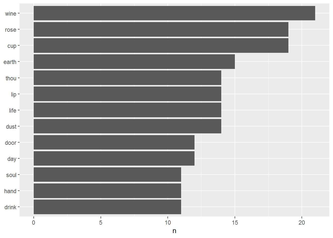
## # … with 1,085 more rowsWine, cup, rose are 3 most common words. In the following, as well, there are words such as earth, dust, life, lip and etc. Well, what are these about? What do the wine and the cup refer to? What about the rose and the lip? and also others.
Maybe, it is obvious. The wine and the cup are referring to binge and having fun. On the other hand, rose is the symbol of lover in Persian poems and of course it has its own complicated means. Then, lip and rose could refer to pleasure and carelessness and of course love. It’s all about seizing the present moment.
Below, words repeated more than 10 times, have been shown.
library(ggplot2)
tidy_khayyam %>%
    count(word, sort = TRUE) %>%
    filter(n > 10) %>%
    mutate(word = reorder(word, n)) %>%
    ggplot(aes(word, n)) +
    geom_col() +
    xlab(NULL) +
    coord_flip()
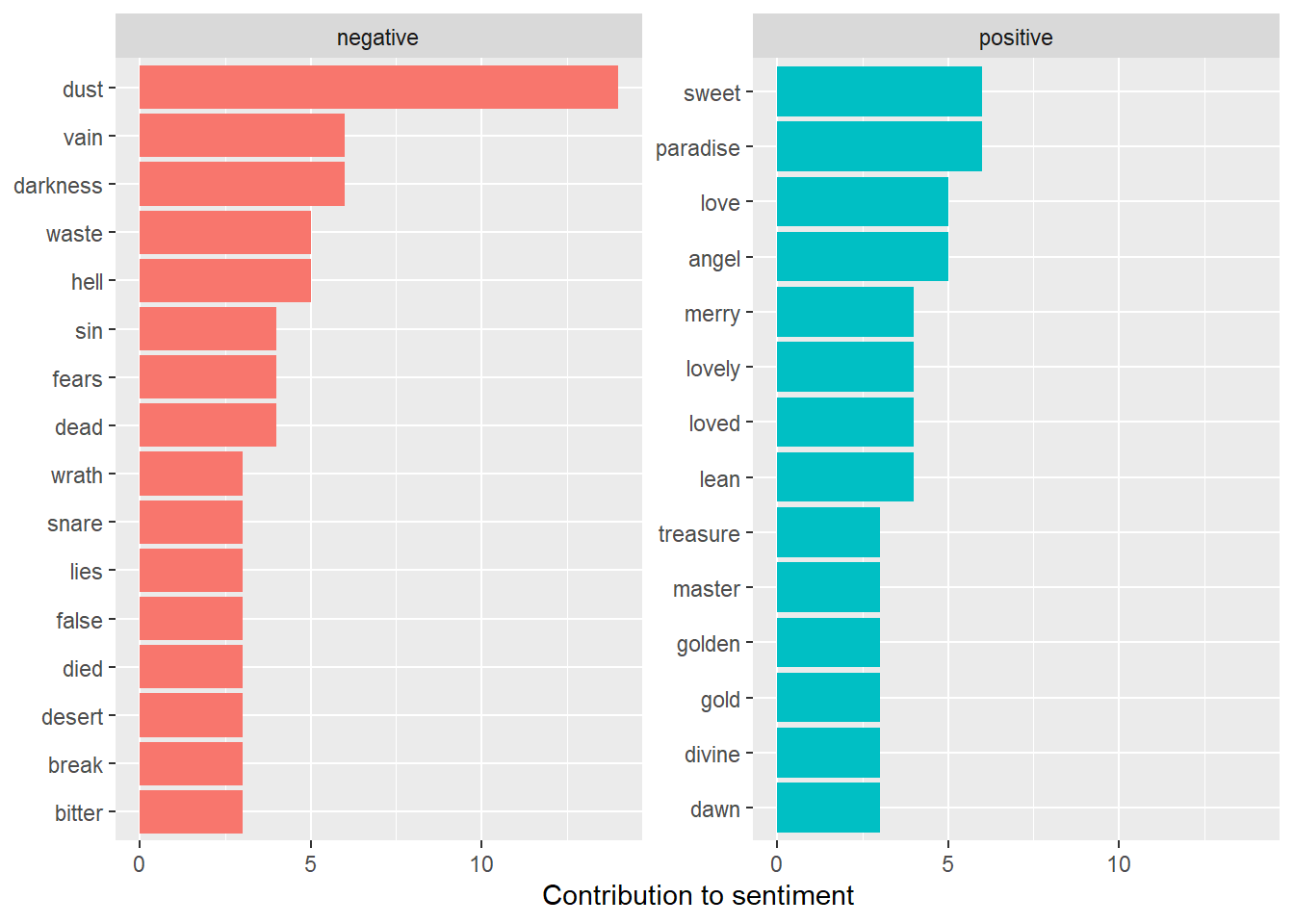
There are some guidelines which can separate the words based on their sentiments. For example positive words or negative words. One of these guidelines is bing.
bing_word_counts <- tidy_khayyam %>%
    inner_join(get_sentiments("bing")) %>%
    count(word, sentiment, sort = TRUE)
## Joining, by = "word"bing_word_counts## # A tibble: 173 × 3
## word sentiment n
## <chr> <chr> <int>
## 1 dust negative 14
## 2 darkness negative 6
## 3 paradise positive 6
## 4 sweet positive 6
## 5 vain negative 6
## 6 angel positive 5
## 7 hell negative 5
## 8 love positive 5
## 9 waste negative 5
## 10 dead negative 4
## # … with 163 more rowsHere, these words have been visually shown.
# This can be shown visually
bing_word_counts %>%
    group_by(sentiment) %>%
    top_n(10) %>%
    mutate(word = reorder(word, n)) %>%
    ggplot(aes(word, n, fill = sentiment)) +
    geom_col(show.legend = FALSE) +
    facet_wrap(~sentiment, scales = "free_y") +
    labs(y = "Contribution to sentiment",
         x = NULL) +
    coord_flip()
## Selecting by n
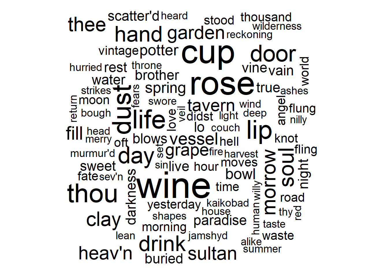
We can check wordcloud plot for Khayyam’s poems. Size of words have been determined based on their frequency.
library(wordcloud)## Loading required package: RColorBrewertidy_khayyam %>%
anti_join(custom_stop_words) %>%
count(word) %>%
with(wordcloud(word, n, max.words = 100))## Joining, by = "word"## Warning in wordcloud(word, n, max.words = 100): round could not be fit on page.
## It will not be plotted.## Warning in wordcloud(word, n, max.words = 100): earth could not be fit on page.
## It will not be plotted.
Topic modeling
Every document could be separated to different topics that each of them may have their own labels. Topic modeling is a method which can be used for this purpose. A popular topic modeling is Latent Dirichlet allocation (LDA). Based on LDA each document is a mixture of topics and each topic is a mixture of words. In Khayyam’s poems, we hypothesize that it contains two different topics; however we can consider more topics too. But, if you are dealing with a document that include several chapters, you can set number of chapters as number of topics.
First of all, we must get the data ready to fit LDA model.
q = tidy_khayyam %>%
     count(gutenberg_id,word, sort = TRUE)
b = q %>%
     cast_dtm(gutenberg_id, word, n)
Now, it’s time to fit LDA with k = 2 (two topics).
ap_lda <- LDA(b, k = 2, control = list(seed = 1234))
ap_lda
## A LDA_VEM topic model with 2 topics.After fitting the model, we can estimate the per-topic-per-word probabilities, called β (“beta”), from the model. Needless to say that these values indicate the probabilities of that term being generated from that topic.
ap_topics <- tidy(ap_lda, matrix = "beta")
ap_topics
## # A tibble: 2,190 × 3
## topic term beta
## <int> <chr> <dbl>
## 1 1 wine 0.00694
## 2 2 wine 0.0110
## 3 1 cup 0.00978
## 4 2 cup 0.00629
## 5 1 rose 0.0108
## 6 2 rose 0.00522
## 7 1 earth 0.00669
## 8 2 earth 0.00604
## 9 1 dust 0.00342
## 10 2 dust 0.00858
## # … with 2,180 more rowsThe term “wine” has a 0.007 probability of being generated from topic 1, but a 0.01 probability of being generated from topic 2.
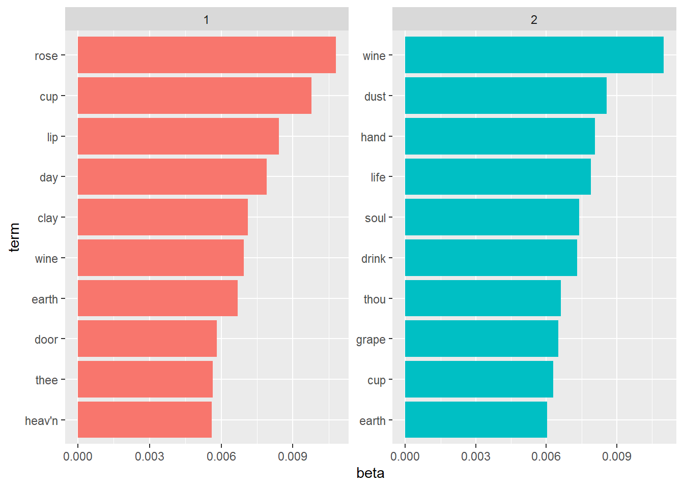
Then we take a look at the 10 terms that are most common within each topic.
ap_top_terms <- ap_topics %>%
     group_by(topic) %>%
     slice_max(beta, n = 10) %>%
     ungroup() %>%
     arrange(topic, -beta)

ap_top_terms %>%
     mutate(term = reorder_within(term, beta, topic)) %>%
     ggplot(aes(beta, term, fill = factor(topic))) +
     geom_col(show.legend = FALSE) +
     facet_wrap(~ topic, scales = "free") +
     scale_y_reordered()
beta_wide <- ap_topics %>%
     mutate(topic = paste0("topic", topic)) %>%
     pivot_wider(names_from = topic, values_from = beta) %>%
     filter(topic1 > .001 | topic2 > .001) %>%
     mutate(log_ratio = log2(topic2 / topic1))
beta_wide
## # A tibble: 544 × 4
## term topic1 topic2 log_ratio
## <chr> <dbl> <dbl> <dbl>
## 1 wine 0.00694 0.0110 0.663
## 2 cup 0.00978 0.00629 -0.636
## 3 rose 0.0108 0.00522 -1.05
## 4 earth 0.00669 0.00604 -0.146
## 5 dust 0.00342 0.00858 1.33
## 6 life 0.00408 0.00790 0.955
## 7 lip 0.00841 0.00338 -1.32
## 8 thou 0.00531 0.00661 0.317
## 9 day 0.00789 0.00218 -1.86
## 10 door 0.00581 0.00435 -0.417
## # … with 534 more rowsIn this output, we see that the term “wine” is more likely to belong to topic 2. On the other hand, terms “cup” and “rose” are more likely to belong to topic 1. Based on the results, we can labels to each of topics, but we don’t do that and leave it to the taste of the dear readers.
Conclusion
We introduced the basics concepts of text mining. Clearly, we didn’t delve into details. In a nutshell, we analyzed the Khayyam’s poems. We saw that Khayyam believes in joy. I highly recommend you to read his poems and personally discover his mindset. If we want to summarize his thought and world view in one sentence, that sentence will be this:
Life is short. Always choose happiness.